Time Series Tokenization Methods for Species Distribution Modelling with Deep Learning
In the context of multi-modal deep learning, this project assessed the improvement in model performance by adding time series as a new modality alongside tabular data. This specific case study was focused on the prediction of plant species distribution in Europe, using the GeoPlant dataset and a transformer architecture. To accomodate for the multi-modal input, each data modality was encoded in a latent space using a tokenizer model before being input in the main transformer, as illustrated in Figure 1. In this project, I implemented and compared four tokenizer model architectures for time series data. The main challenge was to identify a method that effectively represents and captures the temporal structure of time series, which distinguishes them from other types of data. This project is not only relevant to species distribution models and ecology, but also to a wide range of fields such as medical research and financial mathematics, where time series form an integral part of the problems at hand.

Data input and output of model The Geoplant dataset consists of Presence-Absence survey data of plants in Europe, collected by biologists for small observation plots. For each given spatial plot (considered as a point) and survey date, diverse environmental features are provided. They include bioclimatic, soil, elevation, land-cover and human footprints variables, which make up the tabular data. Additionally, for each spatial plot, climatic and satellite 18 years long time series data is available. The time series give insight on the climate and past events that have influenced plant growth, which are absent from the « instantaneous » tabular data. The climatic time series have a monthly resolution and four channels : average precipitation and monthly minimum, maximum and mean temperatures. The satellite time series have a trimestrial resolution and six channels : Red, Green, Blue, near-infrared (NIR) and short-wave infrared 1 and 2 (SWIR1, SWIR2). The model is trained to predict species occurence probability, given the geographical coordinates, the environmental features and the time series features.
A constraint of the time series tokenization method was the preservation of independant weights for each channel. This point was crucial for the evaluation of model performance by selecting specific features during testing and assessing their influence on overall performance, which is possible following the MaskSDM approach presented in 1. Furthermore, the satellite and climatic time series differ in length, necessitating that the tokenization method accommodates variations in input lengths seamlessly. To address these constraints, four architectures are proposed for tokenizing the time series.
- Multilayer Perceptron (MLP) : In MLPs, each internal node attends to all input entries. Even if this model does not account for the temporal structure of the data, the rational for employing it lies in the hypothesis that it may implicitly learn to capture temporal dependencies.
- Fully Convolutional Network (FCN) : Convolutions are known for their ability to exploit spatial correlations in two-dimensional image data. For one-dimensional time series data, the hypothesis is that convolutions with an appropriately defined receptive field can effectively capture meaningful attributes, such as seasonal variations.
- Residual Network (ResNet) : Residual networks utilize residual connections to create shortcuts within each block of CNNs. This capability to capture complex long-term dependencies motivates the use of residual networks for representing temporal dependencies in time series data.
- TransformerEncoder (TE) : As for multilayer perceptrons, the attention mechanism can attend to all tokens of the input data. Additionally, temporality in the input data is explicitly represented by the addition of a positional encoding to each input token.
Firstly, all four Time Series Tokenizer methods are evaluated on the test set to determine which architecture can extract the most meaningful information from the time series data and thus improve the overall multi-modal model performance. The Transformer Encoder demonstrates the highest capacity to extract predictive information from time series. Encoding time series data with the TE leads to an Area Under the Curves (AUC) of 97.6% for the overall model versus 97.5% for the MLP, 97.4% for the FCN and 97.2% for ResNet. For reference, the AUC using only tabular data is 94.7%.
Secondly, to assess the contribution of each time series to the model’s performance, the model is evaluated using only the tabular variables initially, followed by the addition of one type of time series at a time. This approach quantifies the performance improvement resulting from the inclusion of each time series and identifies which type contributes the most. The category that provides the greatest improvement is the RGB satellite time series, increasing the AUC by 2.34% to 97.1%. The other satellite categories also yield significant gains, with AUCs of 97.0% for SWIR and 96.9% for NIR. Climatic time series contribute less to the performance improvement, with the model achieving an AUC of 95.6% when including temperature time series and 95.5% with precipitation time series.
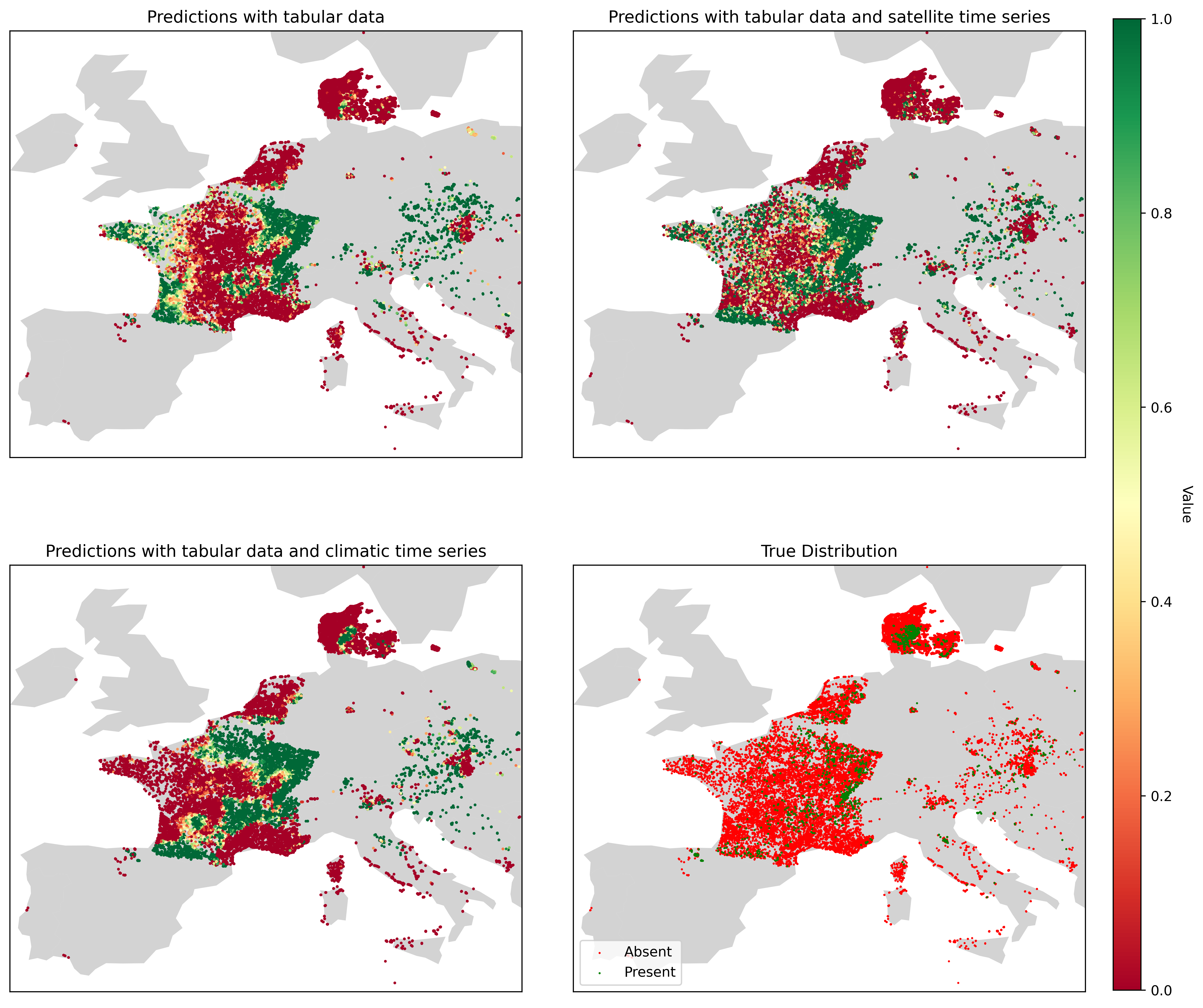
Figure 2 visualizes the differences in model predictions for a specific species under three scenarios: (a) using only tabular data, (b) using tabular data and satellite time series, and (c) using tabular data and climatic time series. Panel (d) provides a comparison with the actual distribution of the species.
The performed experiments demonstrated the valuable addition of information by time series to the deep learning model. In particular, when tabular data is already utilized, the addition of satellite time series results in significant performance improvements. This is likely because satellite data is entirely absent from the tabular dataset. Additionally, time series data alone outperform tabular data when used independently. This is likely because tabular indices, such as those for human footprint or landcover, are derived from aggregated data of lower quality. This underscores the importance of high-quality raw data in deep learning, as models often generate better feature representations than those provided by pre-aggregated indices. Finally, among the four Time Series Tokenizer methods, the Transformer Encoder demonstrates the best performance. This architecture shows great promise in time series embedding, as it effectively captures a large context size while preserving the temporal structure of the input data through the addition of positional encodings.
This project was an opportunity to reflect on the relationship between data structure and the choice of an appropriate model for extracting meaningful information. From a programming perspective, it also helped me gain confidence in implementing different models in PyTorch, including building a transformer encoder from scratch to preserve channel independence.
Download my project report.
-
Zbinden, R., Tiel, N.v., Sumbul, G., Kellenberger, B., Tuia, D. (2025). MaskSDM: Adaptive Species Distribution Modeling Through Data Masking. In: Del Bue, A., Canton, C., Pont-Tuset, J., Tommasi, T. (eds) Computer Vision – ECCV 2024 Workshops. ECCV 2024. Lecture Notes in Computer Science, vol 15624. Springer, Cham. https://doi.org/10.1007/978-3-031-92387-6_14 ↩